Summary: R offers a handful of packages to automate building models. rpart, randomForest, MASS, and forecast packages help you search through a hypothesis space. The caret package helps crawl through the hyper parameter space.
Before I get into how you can automatically build models in R, I’d like to explain what some of the issues are so that you can keep an eye open. It’s important that you use model automation as a tool and not necessarily as the final solution without exploring the data and model assumptions.
Jelly Beans, Overfitting, and Nothing Learned
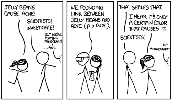
A big risk that you run with automating your model development is that you could find spurious relationships in the data. Like in the above XKCD comic, if you run 20 different tests, there’s a 5% chance you’ll find a significant result just from random chance!
There’s also a chance that you might overfit the training data as your model automation marches toward some optimization metric. Most model automation uses some criteria like AIC or Cross Validation in order to make sure the model is not growing too complex and still has predictive power on test data. The caret package allows for repeated cross validation of the hyper parameter space.
Lastly, a softer but serious concern is that you might not learn anything from letting an algorithm determine your model. Struggling with the data and the model creation helps generate more ideas! The same thing can be said for your understanding of the algorithms you’re working with. If you’re running stepwise regression, you might not realize that a regression tree might be a better option.
Enough warnings. Let’s start programming.
Model Automation Packages in R
In model automation, we either try different variables, different coefficients, or different hyper parameters.
Most of the time you’re trying to optimize for some metric and you iterate over many different configurations. This is similar to how some variable importance methods work.
I will walk through a few methods using the Bank Marketing data set among other packaged data sets.
Decision Trees and Random Forests
A decision tree is a great example of variable importance. The decision tree uses splitting criterion like Gini Index and Entropy. A random forest does the same process but with hundreds of decision trees.
#http://archive.ics.uci.edu/ml/datasets/Bank+Marketing
data <- read.csv("~/in/bank/bank-full.csv",header=T,
         sep=";")

####Decision Tree####
library(rpart)
library(rpart.plot)

rp <- rpart(y~., data = data)
rpart.plot(rp)

####Random Forest Models####
library(randomForest)
rf <- randomForest(y~., data = data)
rf$importance #Var Name + Importance
varImpPlot(rf) #Visualization
Stepwise Regression
Regression requires you to add variables into your model and you test each one to see whether it is significantly different than zero. Stepwise regression allows you to either…
- Forward: Start with a simple model and automatically add variables to it.
- Backward: Start with a complex model and automatically remove variables from it.
- Both: Iterativly add or remove variables each step.
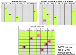
The MASS package offers the stepAIC function. It’s important that you know which direction you will “step”. If you’re moving forward, you will have to create a “lower bound” model which is just the intercept.
If you’re moving backward, you need to create a fully expressed model. Unfortunately, you can’t use the classic Y~.. You’ll see that we use formula(paste()) to get the upper bound of the model.
####Step Wise Regression####
data("mtcars")
mt <- mtcars
#Get the Independent Variables
#(and exclude hp dependent variable)
indep_vars <-paste(names(mt)[-which(names(mt)=="hp")],
                   collapse="+")
#Turn those variable names into a formula
upper_form = formula(paste("~",indep_vars,collapse=""))
#~mpg + cyl + disp + drat + wt + qsec + vs + am + gear + carb

library(MASS)
mod <- lm(hp~.,data=mt)
#Step Backward and remove one variable at a time
stepAIC(mod,direction = "backward",trace = T)
#Create a model using only the intercept
mod_lower = lm(hp~1,data=mt)
#Step Forward and add one variable at a time
stepAIC(mod_lower,direction = "forward",
        scope=list(upper=upper_form,lower=~1))
#Step Forward or Backward each step starting with a intercept model
stepAIC(mod_lower,direction = "both",
        scope=list(upper=upper_form,lower=~1))
auto.arima
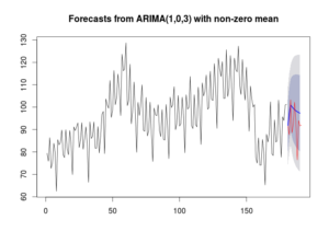
Time series models can be complicated but the forecast package allows you to rapidly produce an ARIMA model. There’s a lot of detail on how it works in the OTexts textbook. Personally, I have used this tool to quickly develop ARIMA models and they have had great results with error around less than 1%.
library(forecast)
library(fpp) #Just to get the data
#Step Backward and remove one variable at a time
data("elecequip")
ee <- elecequip[1:180]
model <- auto.arima(ee,stationary = T)

plot(forecast(model,h=10))
lines(x = 181:191, y= elecequip[181:191],
      type = 'l', col = 'red')
caret package
The caret package in R does a search across a hyper parameter space. Many models require you to set a hyper parameter that influences the training of the model. For example…
- Number of hidden layers in a neural network.
- Number of trees and random variables in random forests.
- Complexity parameter in decision trees.
The caret package allows you to rapidly work through these possible hyper parameters in a simple and even parallel fashion. The main function is train. In the example below, we set up cross validation (10 folds and repeated 10 times) and searching a hyper parameter space of a decision tree with a complexity parameter between 0.0 and 0.01 for every 0.001 steps.
library(caret)
#Step Backward and remove one variable at a time
tctrl <- trainControl(method = "cv",number=10,
                      repeats=10)
#Declare exactly which parameters you want to test
rpart_opts <- expand.grid(cp = seq(0.0,0.01, by = 0.001))

rpart_model <- train(y~., data = data, method="rpart",
                     metric = "Kappa", trControl = tctrl,
                     tuneGrid = rpart_opts)
That’s it! The caret package is incredibly more complicated than what I have presented here. There are dozens of models with many different hyper parameters that you can choose from.


