Summary: Decision trees are used in classification and regression.  One of the easiest models to interpret but is focused on linearly separable data.  If you can’t draw a straight line through it, basic implementations of decision trees aren’t as useful.

A Decision Tree generates a set of rules that follow a “IF Variable A is X THEN…” pattern.  Decision trees are very easy to interpret and are versatile in the fact that they can be used for classification and regression.  A decision tree follows these steps:

• Scan each variable and try to split the data based on each value.
• Split: Given some splitting criterion, compare each split and see which one performs best.
• Repeat the two steps above for each node, considering only the data points in each node.
• Pre-Pruning: Stop partitioning if the node is too small to be split, any future partition is too small, or cross-validation data shows worse performance.
• Post-Pruning: Alternatively, trim the decision tree by removing duplicate rules or simplifying rules.

Split Criteria

There are a handful of different options that have different effects on how your data is partitioned.

• Misclassification Error: Does the split make the model more or less accurate?
• Gini Index: Favors large partitions.  Uses Squared class probabilities.
• Information Gain: Favors smaller partitions.  Uses the base-two log of the class probabilities.
• Gain Ratio: Normalizes Information Gain to penalize many small splits.
• ANOVA: Used in Regression Trees.  Minimizes the variance in each node.

Recursive Partitioning

The implementation of decision trees is a recursive algorithm.  Each iteration, the data is split into smaller chunks and the algorithm is called again on that smaller chunk.  Thus, it is recursive (the algorithm calls itself).

Pre-Pruning Techniques

If you let the recursive nature of decision trees run wild, you’ll end up with a set of rules that have completely overfit your training data – the rules learned won’t be of any use on new data.  In order to prevent that, you can take measures to pre-prune your decision tree.

• Minimum Parent Node Size: What’s the smallest a parent node can be?
• Minimum Split Size: How small are you willing to make a terminal node?
• Cost Complexity: Is adding another node worth it?

Post-Pruning Techniques

Even the best safeguards from overfitting can still develop an overly complicated tree.  One branch might be a duplicate of another branch or the decision tree may have grown exceptionally deep.

• Remove redundant rules: Sometimes a rule might repeat itself.  This adds little value and makes a more complicated tree.
• Cut to a certain depth: The tree may have overfit the training data and build an overly complex model.  Sometimes you need to roll the model back a few branches.

You can use a testing set to identify which branches being removed worsen or improve the model’s performance.

Drawbacks of Decision Trees

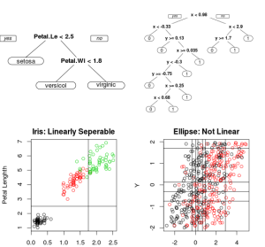
The Iris data set shows very clear linear separation. Compare that to a slightly overlapping pair of ellipses.

• Linearly Separable Rules: The biggest drawback of using a Decision Tree is that it needs linearly separable data points.  That means a Decision Tree can only use straight lines through the data, one variable at a time.
  • Note: To work around this, you could create combinations of your variables or use some data-reduction methods like PCA.

In the example image, you can see that the Iris data set is very easily separated with straight lines.  The colors show the three different classes and two straight lines takes care of the majority of the classifications.

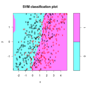
However, if you try using a decision tree on something with an angle, you’ll end up developing many more rules.  The chart and tree on the right side gives a great example of this.  It would be much easier to separate the classes with a diagonal line.  Using Support Vector Machines, it’s more plain to see the real relationship between the two classes.

Follow these steps when building a decision tree and you’ll build generalizable models that make sense.

Advanced Topics

If you know about the splitting criteria and the methods of selecting and evaluating a decision tree, you’re fully capable of using them. For those interested, here are some advanced concepts that separate you from the rest of the crowd.

Surrogate Variables / Splits

An important element of decision trees is the creation of surrogate variables. In the original Breiman paper, he details out how these surrogates can be used to help deal with missing data and identify variable importance.

When a split is made, it depends on one variable. What happens if that variable is missing? Let’s say your working on predicting whether customers will be kept or lost next year.

• A Surrogate Split tries to predict your actual split.
• Another decision tree is created to predict your split.
• In our example, another decision tree would be created to predict Orders <= 6.5 and Orders >= 6.5.
• Using that “fake” decision tree, for any record with the orders missing will be guided to the “correct” direction based on the surroage.
• If the record is missing the surrogate variable, another surrogate is looked for.
• If the surrogate splits can’t beat the “go with the majority” rule, then it’s not considered as a surrogate.

The more you dig into decision trees, the more they do! Granted, it depends on the implementation. The implementation in R makes use of surrogate splits but it looks like the Python implementation does not (based on its feature importance description)

Variable Importance

The very nature of a decision tree reveals “important” variables. Those variables that make it to the top, tend to be the more important variables when explaining your dependent variable.

However, we can quantify this in a couple ways.

• Using Surrogate Splits: Add up the improvement for each time the variable is used as the primary split and then all the times it’s used as a surrogate (but weighted).
• Decrease in Node Impurity: Without using a surrogate split, for large trees (and random forests) you can add up how much each split decreased the node impurity.

Related Links

• Example of Gini Index and Information Gain.
• Review of foundational Classification and Regression Trees book.